 Timing is everything for your sensors. A sensor that is too sluggish to respond to quickly changing levels or pressure won’t alert you to dangerous process conditions until it’s too late. And an overly sensitive sensor sees an emergency in every stray reading or transient condition. Neither sensor is effective, in terms of time or money.
Sensors using sample buffers for signal processing can condition Output Readings using various combinations of four settings: Sample Rate, Averaging, Window, and Out of Range Samples. All four work together to produce an Output Reading customized to your liking. Let’s take a look at them individually, and then look at an admittedly staged example to see their cumulative efforts.
The Sample Rate for a sensor or signal processor is the number of readings evaluated for entry into the sample buffer in a given amount of time, usually expressed in Hz (samples per second). For ultrasonic sensors, this governs how often the sensor “listens” to the sound waves being received by the transducer. For pressure transducers and magnetostrictive sensor that produce continuous readings, the sample rate more accurately describes how often the raw electrical output is sampled by the controlling electronics.
Those samples are then placed in a First In, First Out Averaging buffer. The size of the buffer, in number of samples, is set by you, the user. The contents of the buffer, as advertised by its name, are averaged to produce the output reading. Thus, a smaller buffer will produce a more responsive and perhaps volatile output reading, while a larger buffer generates a smoother reading that is slower to react to changes.
We’ll treat Window and Out of Range Samples together, since they combine to throw the biggest wrench, or softest blanket, on all the backstage math between the sample readings and your sensor’s output reading. Window defines a range of acceptability for sample readings, usually defined in +/- X units from the current output reading. An example would be an ultrasonic sensor on 15’ tall tank, with a current level reading of 6’. A window of +/- 2’ would prevent the reading from jumping from 6’ to 10’.
Out of Range Samples is a First In, First Out buffer, similar to the Averaging buffer. However, it is only for consecutive samples that have been rejected because they fall beyond the range establish by Window. Here’s the wrench I mentioned above: when the Out of Range Samples buffer is filled with consecutive samples, those samples immediately over write the contents of the Averaging buffer, instantly correcting the Output Reading.
The effect is similar to that of the Averaging buffer. A smaller Out of Range Samples buffer allows for a more quickly correcting, and thus chaotic, output reading. A larger Out of Range Samples buffer necessitates a steadier reading beyond the Window in order to move the output reading.
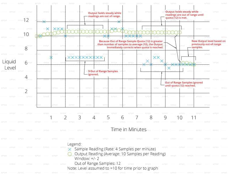
Buffers and Samples and Windows, oh my! Let’s put a visual on these concepts so we can see them in action. As noted at the beginning, this example is staged in order to show all of the settings working with, and against, each other. Thus, the time shown is in minutes, not seconds, and the level readings look a bit ridiculous. The things we do for the sake of easier math.
 The graph to the right illustrates example readings. It shows how Averaging, Sample Rate, Window, and the Out Of Range Samples settings work together to filter out unwanted samples until they become consistent. While this can stop erroneous readings, it also slows down the response time to legitimate change.
As the legend calls out, the level reading is being sampled four times every minute (or every 15 seconds), the Averaging buffer is set to 10 readings, the Window is +/- 2 units, and the Out of Range Samples buffer is set to 12 readings.
Because the buffers are set to 2.5 and 3 times the sample rate (10 and 12 versus four), the Output Reading is very stable compared to the Sample Readings. Thus, two minutes of Out of Range level samples are ignored, but after three minutes of Out of Range Samples, the Output Reading corrects by more than four units, even though the Window is set to two units.
These ratios of these four settings can be fine-tuned to fit the specific scenario of your application. For an ultrasonic over a tank with regular intervals of turbulence, few samples per second and/or larger Averaging and Out of Range buffers can mitigate the anticipated effects of that turbulence on the output reading. Conversely, a sensor monitoring a liquid level prone to sudden increases or decreases (large volume inputs, outputs) would probably be better served with more frequent samples and a smaller Window and buffers so that the Output Reading accurately reflects the quick changes.
Not sure how to best adjust your sensor’s settings to match your application? Our Measurement Experts would love to help maximize the meaningful output of your sensor. Contact them today!